Advanced Search
Volume 40 Issue 4
Aug.  2022
Turn off MathJax
Article Contents

DONG XiaoLong, HU XiuMian, GUO RongHua, LAI Wen. Comparative Experimental Research on Detrital Statistics of River Sand[J]. Acta Sedimentologica Sinica, 2022, 40(4): 871-882. doi: 10.14027/j.issn.1000-0550.2021.099
Citation: DONG XiaoLong, HU XiuMian, GUO RongHua, LAI Wen. Comparative Experimental Research on Detrital Statistics of River Sand[J]. Acta Sedimentologica Sinica, 2022, 40(4): 871-882. doi: 10.14027/j.issn.1000-0550.2021.099

Comparative Experimental Research on Detrital Statistics of River Sand

doi: 10.14027/j.issn.1000-0550.2021.099
Funds:

The Second Tibetan Plateau Scientific Expedition (STEP) Program 2019QZKK0204

  • Received Date: 2021-03-09
  • Rev Recd Date: 2021-07-05
  • Publish Date: 2022-08-10
  • Statistical analysis is the most effective way of determining the component and content of sand or sandstone, and is widely applied in the analysis of terrigenous detritus. Methods include grain counting, the Glagolev-Chayes method, the Gazzi-Dickinson method and the area method. The number of grains to be taken into account in each of these approaches is controversial, and ranges between 300 and 500. The extent to which the statistical result is affected by the sorting degree and grain percentage has not previously been addressed. In this study, two modern river sand samples were collected from the main stream of the Yarlung Tsangpo River for statistical analysis using the four methods, in addition to Matlab simulation statistics. The area method was adopted as the standard which most closely represents the true composition of the sample. It was found that the Glagolev-Chayes method was the most similar to the area method, and the grain-counting method gave the greatest difference. Moreover, poorer sorting of the samples increased the discrepancy between the grain-counting method and the area method, leading to a statistical bias for the components comprising less than 10% of the sample, and the Lv/Lm/Ls diagram is not recommended in this case. The count number is no less than 384 to ensure 95% confidence. Either the area method or the Glagolev-Chayes method is highly recommended rather than the Gazzi-Dickinson method for detrital statistics when calculating river flux.
  • [1] Chayes F. Petrographic modal analysis[M]. New York: John Wiley and Sons, 1956: 113.
    [2] Basu A. Petrology of Holocene fluvial sand derived from plutonic source rocks: Implications to paleoclimatic interpretation[J]. Journal of Sedimentary Petrology, 1976, 46(3): 694-709.
    [3] Suttner L J. Sedimentary petrographic provinces: An evaluation. [C]// Ross C A. Paleogeographic provinces and provinciality. SEPM Special Publication, 1976, 21: 75-84.
    [4] Ingersoll R V, Bullard T F, Ford R L, et al. The effect of grain size on detrital modes: A test of the Gazzi-Dickinson point-counting method[J]. Journal of Sedimentary Petrology, 1984, 54(1): 103-116.
    [5] Garzanti E, Vezzoli G, Andò S, et al. Sand petrology and focused erosion in collision orogens: The Brahmaputra case[J]. Earth and Planetary Science Letters, 2004, 220(1/2): 157-174.
    [6] Fleet W F. Petrological notes on the old red sandstone of the west midlands[J]. Geological Magazine, 1926, 63(11): 505-516.
    [7] van der Plas L. Preliminary note on the granulometric analysis of sedimentary rocks[J]. Sedimentology, 1962, 1(2): 145-157.
    [8] Galehouse J S. Point-counting[M]//Carver R E. Procedures in sedimentary petrology. NewYork: Wiley, 1971: 385-407.
    [9] Glagolev A A. Quantitative analysis with the microscope by the point method[J]. Engineering and Mining Journal, 1934, 135: 399-400.
    [10] Chayes F. A simple point counter for thin-section analysis[J]. American Mineralogist, 1949, 34(1/2): 1-11.
    [11] Garzanti E, Andò S. Heavy minerals for junior woodchucks[J]. Minerals, 2019, 9(3): 148.
    [12] Zuffa G G. Hybrid arenites: Their composition and classification[J]. Journal of Sedimentary Petrology, 1980, 50(1): 21-29.
    [13] Mack G H. Exceptions to the relationship between plate tectonics and sandstone composition[J]. Journal of Sedimentary Petrology, 1984, 54(1): 212-220.
    [14] Palomares M, Arribas J. Modern stream sands from compound crystalline sources: Composition and sand generation index[J]. Geological Society of America Special Papers, 1993, 284: 313-322.
    [15] Garzanti E, Andò S, Vezzoli G. Grain-size dependence of sediment composition and environmental bias in provenance studies[J]. Earth and Planetary Science Letters, 2009, 277(3/4): 422-432.
    [16] Gazzi P. Le arenarie del flysch sopracretaceo dell' Apennino modenese: Correlazioni con il flysch di Monghidoro[J]. Mineralogica et Petrographica Acta, 1966, 12: 69-97.
    [17] Dickinson W R. Interpreting detrital modes of graywacke and arkose[J]. Journal of Sedimentary Petrology, 1970, 40(2): 695-707.
    [18] Lai W, Hu X M, Garzanti E, et al. Initial growth of the northern Lhasaplano, Tibetan Plateau in the early Late Cretaceous (ca. 92 Ma)[J]. Geological Society of America Bulletin, 2019, 131(11/12): 1823-1836.
    [19] Leier A L, DeCelles P G, Kapp P, et al. The Takena Formation of the Lhasa terrane, southern Tibet: The record of a Late Cretaceous retroarc foreland Basin[J]. Geological Society of America Bulletin, 2007, 119(1/2): 31-48.
    [20] 马收先,孟庆任,曲永强. 轻矿物物源分析研究进展[J]. 岩石学报,2014,30(2):597-608.

    Ma Shouxian, Meng Qingren, Qu Yongqiang. Development on provenance analysis of light minerals[J]. Acta Petrologica Sinica, 2014, 30(2): 597-608.
    [21] Ingersoll R V, Bullard T F, Ford R L, et al. The effect of grain size on detrital modes: A test of the Gazzi-Dickinson point-counting method-reply to discussion of Lee J. Suttner and Abhijit Basu[J]. Journal of Sedimentary Petrology, 1985, 55(4): 617-618.
    [22] Garzanti E, Vezzoli G, Senna P, et al. Discriminating source rock and environmental control from detrital modes of Permo-Triassic fluvio-deltaic sandstones: II. Austroalpine domain (Livigno, Italy)[M]//Valloni R, Basu A. Memorie descrittive della carta geologica d'Italia. Volume LXI. quantitative provenance studies in Italy. Roma: Istituto Poligrafico e Zecca dello Stato, 2002.
    [23] Folk R L. A comparison chart for visual percentage estimation[J]. Journal of Sedimentary Petrology, 1951, 21(1): 32-33.
    [24] Terry R D, Chilingar G V. Summary of “Concerning some additional aids in studying sedimentary formations”[J]. Journal of Sedimentary Petrology, 1955, 25(3): 229-234.
    [25] Jerram D A. Visual comparators for degree of grain-size sorting in two and three-dimensions[J]. Computers & Geosciences, 2001, 27(4): 485-492.
    [26] Grove C, Jerram D A. jPOR: An ImageJ macro to quantify total optical porosity from blue-stained thin sections[J]. Computers & Geosciences, 2011, 37(11): 1850-1859.
    [27] Zhang X F, Liu B, Wang J Q, et al. Adobe photoshop quantification (PSQ) rather than point-counting: A rapid and precise method for quantifying rock textural data and porosities[J]. Computers & Geosciences, 2014, 69: 62-71.
    [28] Ingersoll R V. Petrofacies and provenance of Late Mesozoic forearc Basin, northern and central California[J]. AAPG Bulletin, 1983, 67(7): 1125-1142.
    [29] Ma A L, Hu X M, Garzanti E, et al. Sedimentary and tectonic evolution of the southern Qiangtang Basin: Implications for the Lhasa-Qiangtang collision timing[J]. Journal of Geophysical Research: Solid Earth, 2017, 122(7): 4790-4813.
    [30] Folk R L, Ward W C. Brazos river bar: A study in the significance of grain size parameters[J]. Journal of Sedimentary Petrology, 1957, 27(1): 3-26.
    [31] Wald A, Wolfowitz J. Statistical tests based on permutations of the observations[J]. The Annals of Mathematical Statistics, 1944, 15(4): 358-372.
    [32] 孙山泽. 抽样调查[M]. 北京:北京大学出版社,2007: 1-169.

    Sun Shanze. Sampling survey[M]. Beijing: Peking University Press, 2007: 1-169.
  • 加载中
通讯作者: 陈斌, bchen63@163.com
  • 1. 

    沈阳化工大学材料科学与工程学院 沈阳 110142

  1. 本站搜索
  2. 百度学术搜索
  3. 万方数据库搜索
  4. CNKI搜索

Figures(13)  / Tables(2)

Article Metrics

Article views(259) PDF downloads(158) Cited by()

Proportional views
Related
Publishing history
  • Received:  2021-03-09
  • Revised:  2021-07-05
  • Published:  2022-08-10

Comparative Experimental Research on Detrital Statistics of River Sand

doi: 10.14027/j.issn.1000-0550.2021.099
Funds:

The Second Tibetan Plateau Scientific Expedition (STEP) Program 2019QZKK0204

Abstract: Statistical analysis is the most effective way of determining the component and content of sand or sandstone, and is widely applied in the analysis of terrigenous detritus. Methods include grain counting, the Glagolev-Chayes method, the Gazzi-Dickinson method and the area method. The number of grains to be taken into account in each of these approaches is controversial, and ranges between 300 and 500. The extent to which the statistical result is affected by the sorting degree and grain percentage has not previously been addressed. In this study, two modern river sand samples were collected from the main stream of the Yarlung Tsangpo River for statistical analysis using the four methods, in addition to Matlab simulation statistics. The area method was adopted as the standard which most closely represents the true composition of the sample. It was found that the Glagolev-Chayes method was the most similar to the area method, and the grain-counting method gave the greatest difference. Moreover, poorer sorting of the samples increased the discrepancy between the grain-counting method and the area method, leading to a statistical bias for the components comprising less than 10% of the sample, and the Lv/Lm/Ls diagram is not recommended in this case. The count number is no less than 384 to ensure 95% confidence. Either the area method or the Glagolev-Chayes method is highly recommended rather than the Gazzi-Dickinson method for detrital statistics when calculating river flux.

DONG XiaoLong, HU XiuMian, GUO RongHua, LAI Wen. Comparative Experimental Research on Detrital Statistics of River Sand[J]. Acta Sedimentologica Sinica, 2022, 40(4): 871-882. doi: 10.14027/j.issn.1000-0550.2021.099
Citation: DONG XiaoLong, HU XiuMian, GUO RongHua, LAI Wen. Comparative Experimental Research on Detrital Statistics of River Sand[J]. Acta Sedimentologica Sinica, 2022, 40(4): 871-882. doi: 10.14027/j.issn.1000-0550.2021.099
  • 碎屑统计是确定砂或砂岩的物质组成、判定其物源的重要研究方法。通常选取具有代表性的砂或砂岩样品磨制成薄片,在显微镜下进行定量统计。统计方法大致可分为点记法和面积法两类,其中点记法最为常用。

    一般而言,点记法就是通过获得各类型颗粒的点数来代表其相对含量,分析岩屑的成分和比例,并通过Q/F/L三角图来展示[15]。早期地质工作者采取统计薄片中所有或某个区域内的颗粒来获得整个样品的物质组成和相对含量[67]。然而该方法统计工作量大,而且统计的结果不能转化为碎屑组分的面积比[8]。Glagolev[9]和Chayes[1,10]提出用网格节点计数法来统计碎屑颗粒,并由Galehouse[8]系统总结形成完整的Glagolev-Chayes统计方法,该方法获得的统计结果能够转化为相应的面积比[11]。随后,以Basu[2]和Suttner[3]为代表的学者提出,通过筛选出中粒砂来进行碎屑统计才具有意义。这种方法影响了后续的许多学者[1214],然而,这种“窄粒径”范围受等效沉降作用的影响较大,不同粒径的选择性统计会对结果造成较大的偏差[11,15]。随后由Gazzi[16]和Dickinson[17]提出、Ingersoll et al.[4]对其系统总结的Gazzi-Dickinson统计法,对“窄粒径”碎屑统计方法提出了质疑,并明确指出Gazzi-Dickinson统计法不需要对样品粒径进行筛选,对同一样品不同粒径的颗粒进行统计,结果更集中,而传统方法更分散。Gazzi-Dickinson法在基于以薄片为研究对象的碎屑物源分析中发挥了重要作用,被后续研究者的广泛接受和采纳[5,1819],成为砂或砂岩碎屑统计分析的主流方法。然而,也有学者指出Gazzi-Dickinson统计法仅适合用于构造环境分析而不适于气候、搬运历史和成岩作用的解释[4,2021],无法改变水动力分选对统计结果的影响[22]

    面积法早期采用标准对比来近似估计颗粒的面积[2325],然而这种方法受个人因素影响太大,所估计的结果也不够准确。近年来,随着图像分析技术的迅速发展,一些地质工作者利用ImageJ和Photoshop等图像分析软件精确计算显微图片中各颗粒类型的面积[2627],使得获得颗粒面积成为了可能。

    以上两类方法面临的共同问题是,需要统计多少个颗粒才具有代表性。Ingersoll[28]提出的统计数量为500颗,而随后Ingersoll et al.[4]又提出统计数量300颗能够达到统计要求。而现今大多数学者统计400颗以上[5,1819,29]。目前,在碎屑统计中没有一个定量的标准,也缺乏实例的验证和模拟。另一方面,在统计过程中影响统计结果的因素有哪些?是否需要考虑粒径的大小,分选程度对统计结果有何影响。四种不同的统计方法对同一样品的统计结果有何差异性?点记法所得到的统计结果能够代表颗粒的真实面积比吗?这方面的研究和报道也极少。

    本次实验以青藏高原雅鲁藏布江干流的河流砂为研究对象,采用薄片实际统计和Matlab模拟统计两种方法,以期明确不同的统计方法统计结果的差异性,评估颗粒分选程度和颗粒含量对统计结果的影响。用实验统计结果验证统计数量需要达到多少颗时才能够达到统计学要求,以及在统计中应该注意的事项,并针对不同应用场景给出建议统计方法。

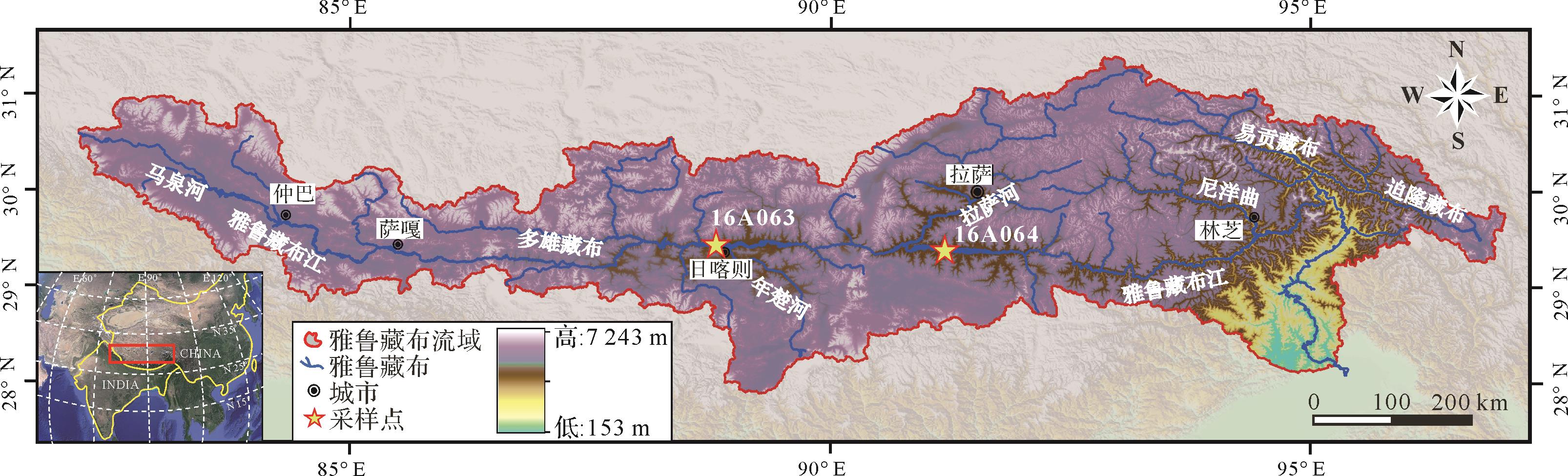
  • 本次研究选用2016年6月采集于雅鲁藏布江干流心滩位置的河流砂样品16A063(日喀则市附近,GPS坐标:29°19′13.5″ N,88°51′28.4″ E)和16A064(拉萨贡嘎机场附近,GPS坐标:29°16'50.00" N,91°10'29.00" E)(图1),用63 μm和2 000 μm的筛网干筛获得粒径在63~2 000 μm的砂样,两个样品在该粒径范围内的质量分别为:16A063为89.3%;16A064为91.5%,代表了主要的物质组分。用分样器均分得到4份样品,每份约2 g。每个样品各磨制标准光学薄片4张供碎屑统计分析。

    Figure 1.  Simplified map of the Yarlung Tsangpo River drainage basin showing locations of studied river sand samples

  • 利用Nikon NIS Elements图像分析软件测量颗粒面积,同时计算每个颗粒的周长、长轴粒径和短轴粒径。本次研究采用长轴粒径作为颗粒粒径,根据公式Ф=-log2D进行单位换算,其中“D”是以毫米为单位的颗粒直径,粒度分选计算公式为:δ Φ=(Ф8416)/4+(Ф955)/6.6,分选可描述为:1) δ Φ<0.35分选很好;2) δ Φ=0.35~0.50分选好;3) δ Φ=0.50~0.71分选中等偏好;4) δ Φ=0.71~1.00分选中等;δ Φ=1.00~2.00分选差;δ Φ>2.00分选极差[30]。计算得出δ Φ(16A063)=0.79,δ Φ(16A064)=0.64。样品16A063共测得粒径个数2 511颗,粒度范围主要为2~4 Ф,粒度中值为3 Ф,以细粒和极细粒为主(图2a);样品16A064共测得粒径个数2 252颗粒度范围主要为1~3 Ф,粒度中值为2.6 Ф,以中细粒为主(图2b)。可知样品16A063分选中等,样品16A064分选中等偏好。

    Figure 2.  Cumulative grain size probability curves and frequency histograms for two studied samples

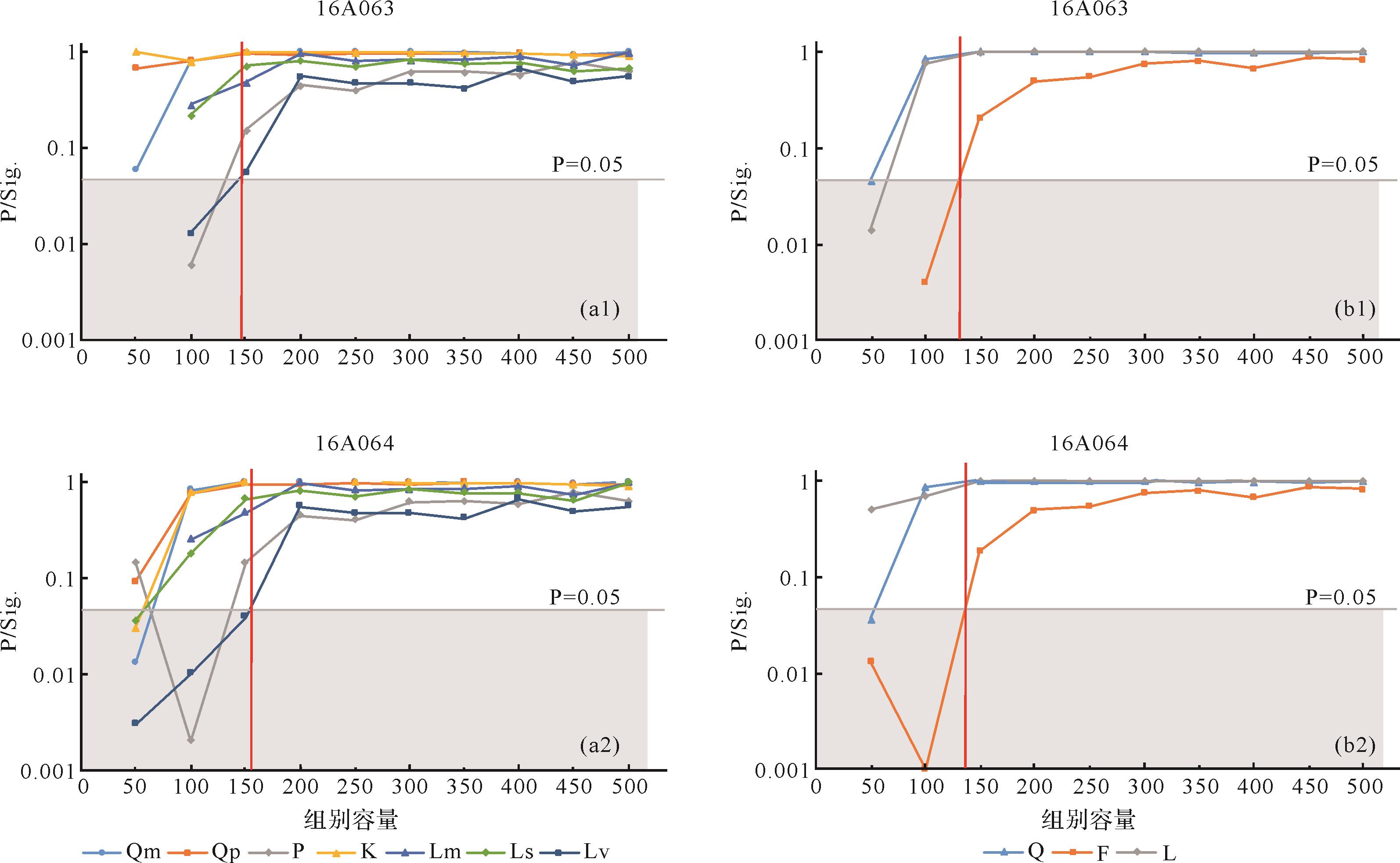
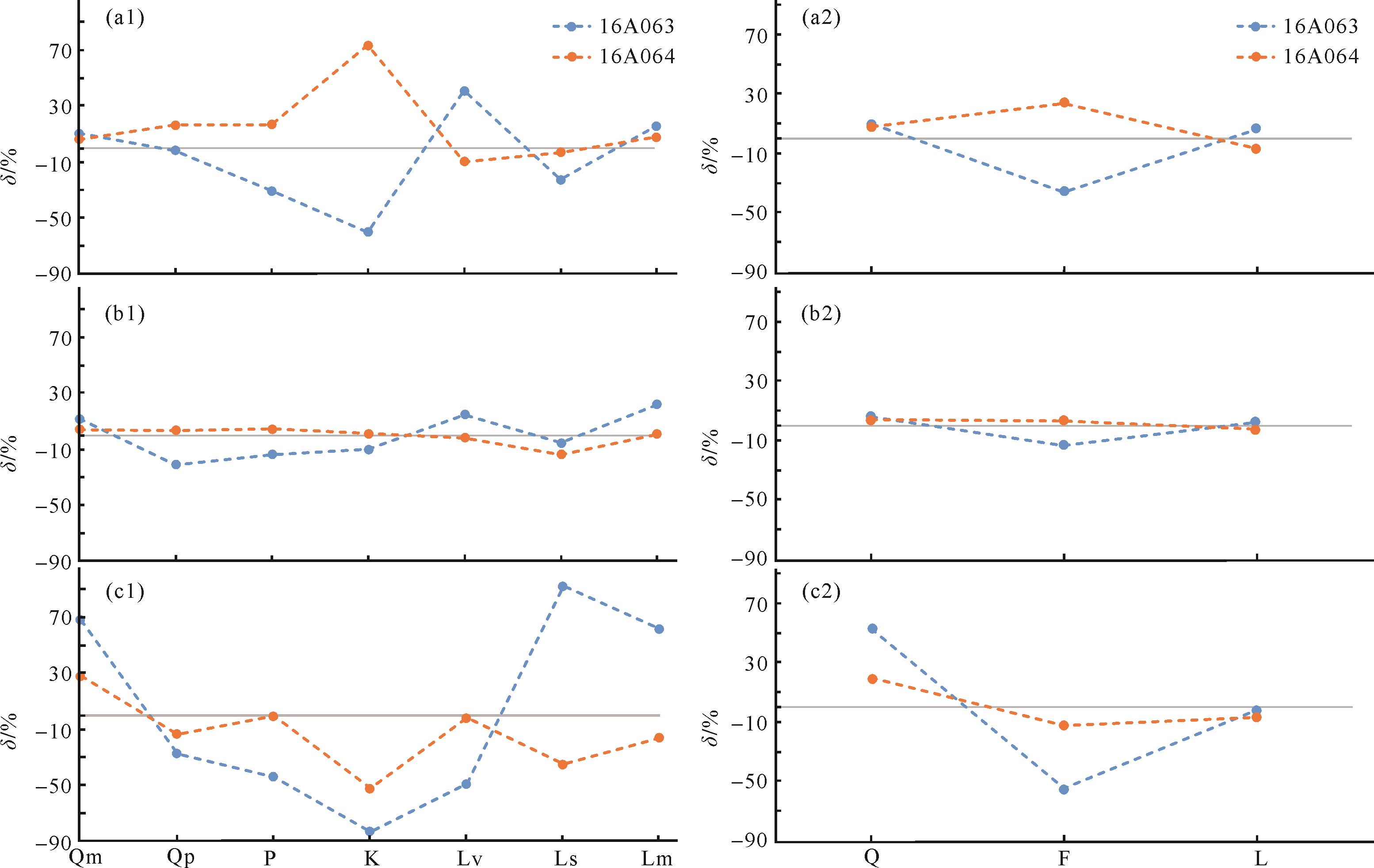
  • 利用IBM SPSS Statistics 26.0软件进行卡方检验来判断样品是否分布均匀。将每张薄片统计的颗粒随机分成不同容量的不同组别,以50为公差递增统计,从0至500颗共11个不同容量的组别,在每个容量内统计出不同类型颗粒百分比,比较各组之间同一类型颗粒的含量百分比变化情况。卡方检验计算得到P值(显著性),当P值均大于0.05,则认为该容量下的颗粒均匀分布。

    样品16A063的组别容量达到150时,该样品内的所有颗粒类型均匀分布(图3a1,b1);样品16A064的组别容量达到200时,该样品内的所有颗粒类型均匀分布(图3a2,b2)。当颗粒容量仅有150颗时,仅有Q/F/L三大类呈现均匀分布。两个样品随机选取的颗粒大于200颗时,该容量内的7小类颗粒均匀分布。因此,从统计的角度来看,只要统计的颗粒数大于200颗,这两个样品都达到均匀分布的要求。

    Figure 3.  SPSS chi⁃squared test of uniform grain distribution

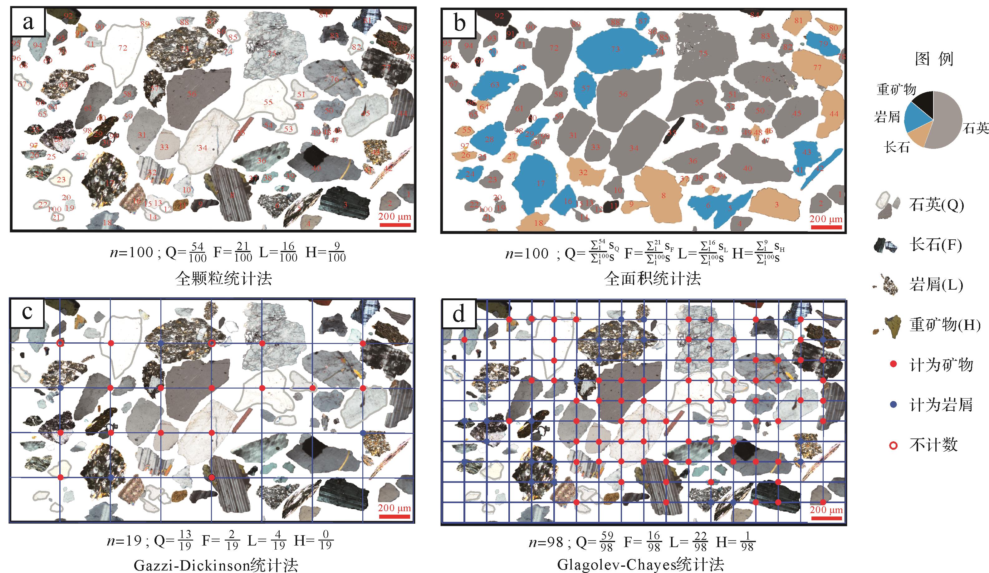
  • 挑选混合均匀的薄片16A063和16A064各一张。对同一薄片采用具有代表性的四种统计方法(全颗粒法、全面积法、Gazzi-Dickinson法和Glagolev-Chayes法)进行统计,具体方法介绍如下。

  • 颗粒统计法包括全颗粒统计法和Gazzi-Dickinson法。

    全颗粒统计法:在偏光显微镜下,对载玻片上一定区域内的所有颗粒逐一进行鉴定并统计,然后将统计的各类型的颗粒的数量换算后,得到各颗粒类型的百分含量(图4a)。

    Figure 4.  Four different detrital statistical methods

    Gazzi-Dickinson统计法:需要选择合适的栅格,栅格间距大于最大砂粒直径以避免重复计数。对落在栅格结点上粒径大于62.5 µm的颗粒进行鉴定并计数,落在基质或胶结物上不计数。若一个大于62.5 µm的矿物颗粒包含在岩屑中则单独计数。例如,玄武岩岩屑中>62.5 µm的斜长石斑晶位于栅格结点上时,则需要标记为长石而不是岩屑[4]图4c)。

  • 面积统计法包括全面积统计法和Glagolev-Chayes法。

    全面积统计方法:利用Nikon NIS Elements图像分析软件进行统计,对颗粒类型进行鉴定,然后手动描出每一个颗粒边界,获得每个颗粒的类型和对应的面积,最终得到薄片中每种颗粒类型的总面积,然后换算成百分比(图4b)。

    Glagolev-Chayes统计法:同样是选择合适的栅格,将网格间距设置成小于颗粒的平均粒径,对落在粒径大于62.5 µm的碎屑颗粒上的网格节点均计数。落在基质或胶结物上的点则不计数。用于重矿物统计则根据实际粒径大小,选取合适的网格(图4d)。如Garzanti et al.[11]对粒径15~500 µm的重矿物统计时选取的网格间距为125 µm。这种方法统计的节点数与颗粒的大小成正比,用节点数的多少来代表面积的大小,统计的结果能够转化为相应的面积百分比。

    为了定量描述全颗粒法、Gazzi-Dickinson统计法、Glagolev-Chayes统计法和全面积法统计结果的差异性,采用这四种方法对同一样品进行统计,对比统计结果。

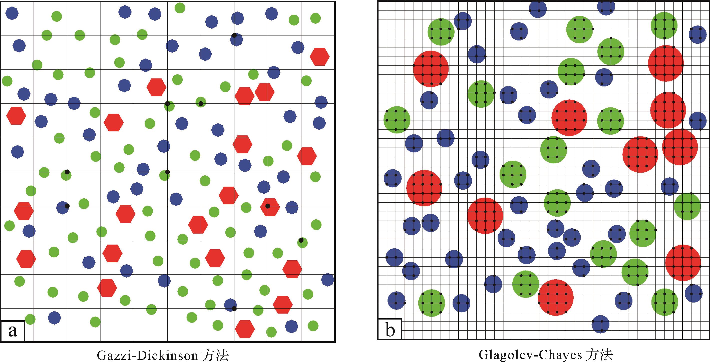
  • 为了更好地评估以上两类统计方法,基于Matlab编写的程序(附件),模拟显微镜下的碎屑统计过程。在Matlab中随机生成颜色不同的圆或任意多边形,设置颗粒随机分布,调整不同颗粒间面积的相对比例和粒径大小等参数,来模拟在已知面积或者颗粒比例的情况下,用Gazzi-Dickinson统计法和Glagolev-Chayes统计法分别进行统计(图5),评估不同因素对抽样统计结果和实际情况的偏差。

    Figure 5.  Matlab simulation of Gazzi⁃Dickinson and Glagolev⁃Chayes statistical methods

    设置等粒径等面积、等粒径不等面积、不等粒径等面积和不等粒径不等面积四种情况,模拟采用全颗粒法和Gazzi-Dickinson法同时对这四种不同情况下的红、绿、蓝三色小球进行统计,以及模拟全面积法和Glagolev-Chayes法同时在这四种情况下的统计。

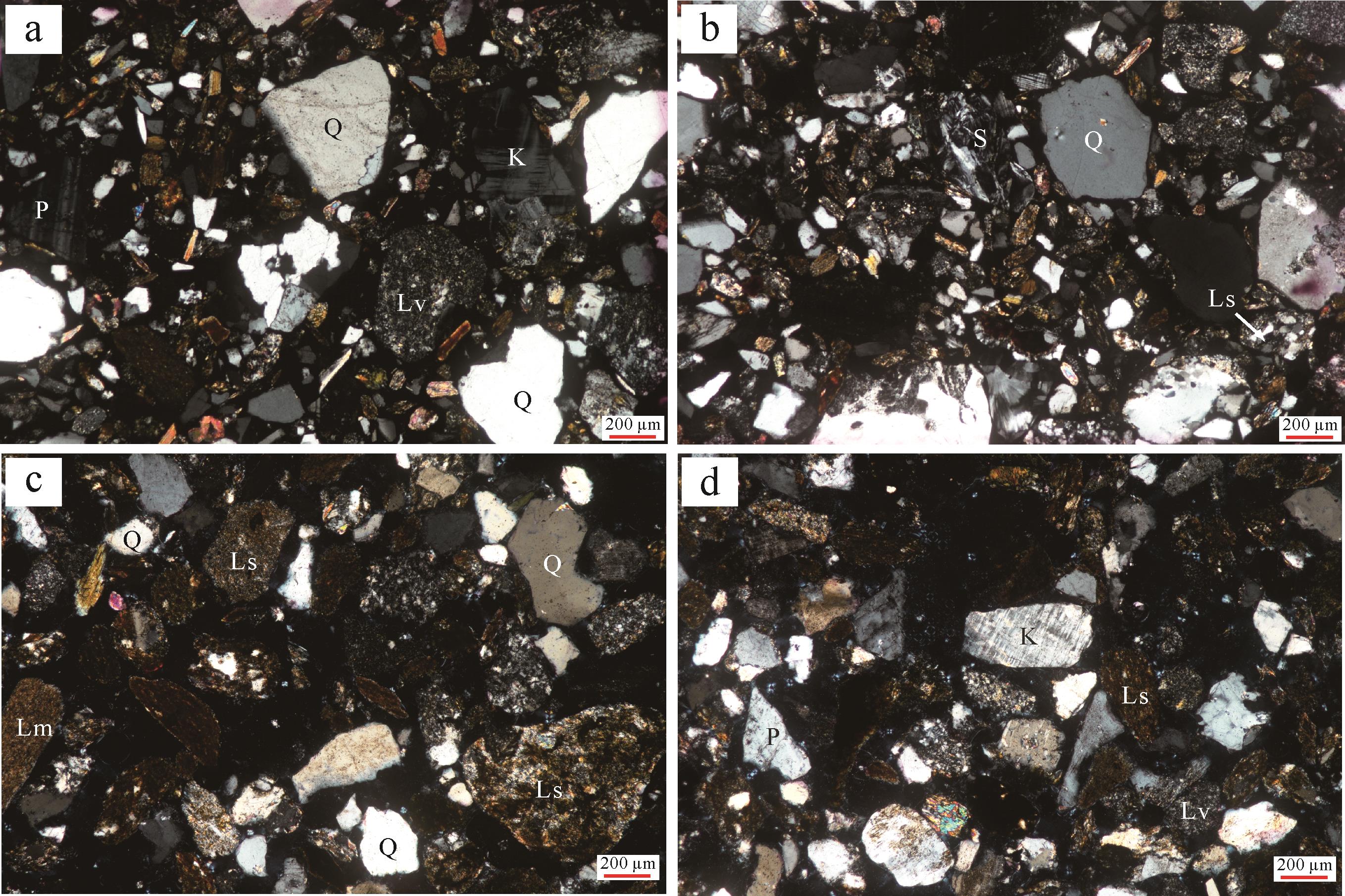
  • 采用全颗粒法(颗粒法)、全面积法(面积法)、Gazzi-Dickinson法(G-D法)和Glagolev-Chayes法(G-C法)统计的结果显示,样品16A063的Q/F/L比例分别为:45∶12∶44;29∶26∶45;41∶18∶41;31∶23∶46;Ls/Lv/Lm的比例分别为:19∶14∶11;10∶28∶7;13∶19∶9;11∶27∶8(图6a,b、表1)。样品16A064的Q/F/L比例分别为:45∶12∶44;29∶26∶45;41∶18∶41;31∶23∶46;Ls/Lv/Lm的比例分别为:34∶7∶59;28∶9∶63;36∶9∶55;29∶9∶62(图6c,d、表1)。

    Figure 6.  Photomicrographs illustrating the variation in the composition of sand from the Yarlung Tsangpo River

    样品 统计方法 颗粒数 Qm Qp P K Ls Lv Lm total Qp/Q P/K Q/(F+L) Q F L
    16A063 颗粒法 2 511 41 3 10 1 19 14 11 100 7 837 81 45 12 44
    面积法 2 511 25 5 19 7 10 28 7 100 16 250 41 29 26 45
    G-D法 431 37 3 15 3 13 19 9 100 8 483 69 41 18 41
    G-C法 1 892 28 4 16 7 11 27 8 100 12 240 45 31 23 46
    16A064 颗粒法 2 252 29 5 7 1 48 3 7 100 15 726 51 34 7 59
    面积法 2 252 22 6 7 2 50 5 8 100 21 347 39 28 9 63
    G-D法 614 30 6 8 2 44 3 8 100 16 489 57 36 9 55
    G-C法 1 620 23 6 7 2 49 5 8 100 21 358 42 29 9 62

    Table 1.  Statistical results for samples 16A063 and 16A064 using the four methods (%)

  • 同时采用人工统计和模拟统计,用全颗粒法与Gazzi-Dickinson方法统计的结果进行对比,比较这两种方法的差异性。

  • 采用全颗粒法与Gazzi-Dickinson法对两个样品分别进行统计,样品16A063中两种方法的偏差范围为-83%~92%,样品16A064两种方法的偏差范围为-52%~27%(图7a1,a2、表2)。两个样品无论是大类还是小类均表现出较大的偏差,说明Gazzi-Dickinson法统计结果并不代表该区域内的所有颗粒的统计结果,是由于两种方法本身的差异所造成的,如将含有大于62.5 μm斑晶的岩屑进行分解。

    Figure 7.  Deviation of the four statistical methods

    颗粒类型 δ(颗粒法-面积法)/面积法 δ(G-D法-颗粒法)/颗粒法 δ(G-C法-面积法)/面积法
    16A063 16A064 16A063 16A064 16A063 16A064
    Qm 67.78% 27.76% 10.42% 6.28% 11.75% 4.34%
    Qp -27.47% -13.68% -1.60% 16.55% -20.98% 3.57%
    P -44.12% -0.66% -30.77% 16.94% -13.56% 4.53%
    K -83.31% -52.52% -60.03% 73.74% -9.97% 1.23%
    Ls -49.05% -2.18% 41.09% -9.66% 14.85% -1.75%
    Lv 92.19% -35.38% -22.52% -3.21% -5.45% -13.58%
    Lm 61.61% -16.47% 15.74% 8.02% 22.31% 1.00%
    Q 52.84% 19.07% 9.43% 7.84% 6.61% 4.18%
    F -55.32% -12.26% -35.79% 23.82% -12.54% 3.79%
    L -2.18% -6.86% 6.49% -7.19% 3.01% -2.38%

    Table 2.  Deviations of the four different methods

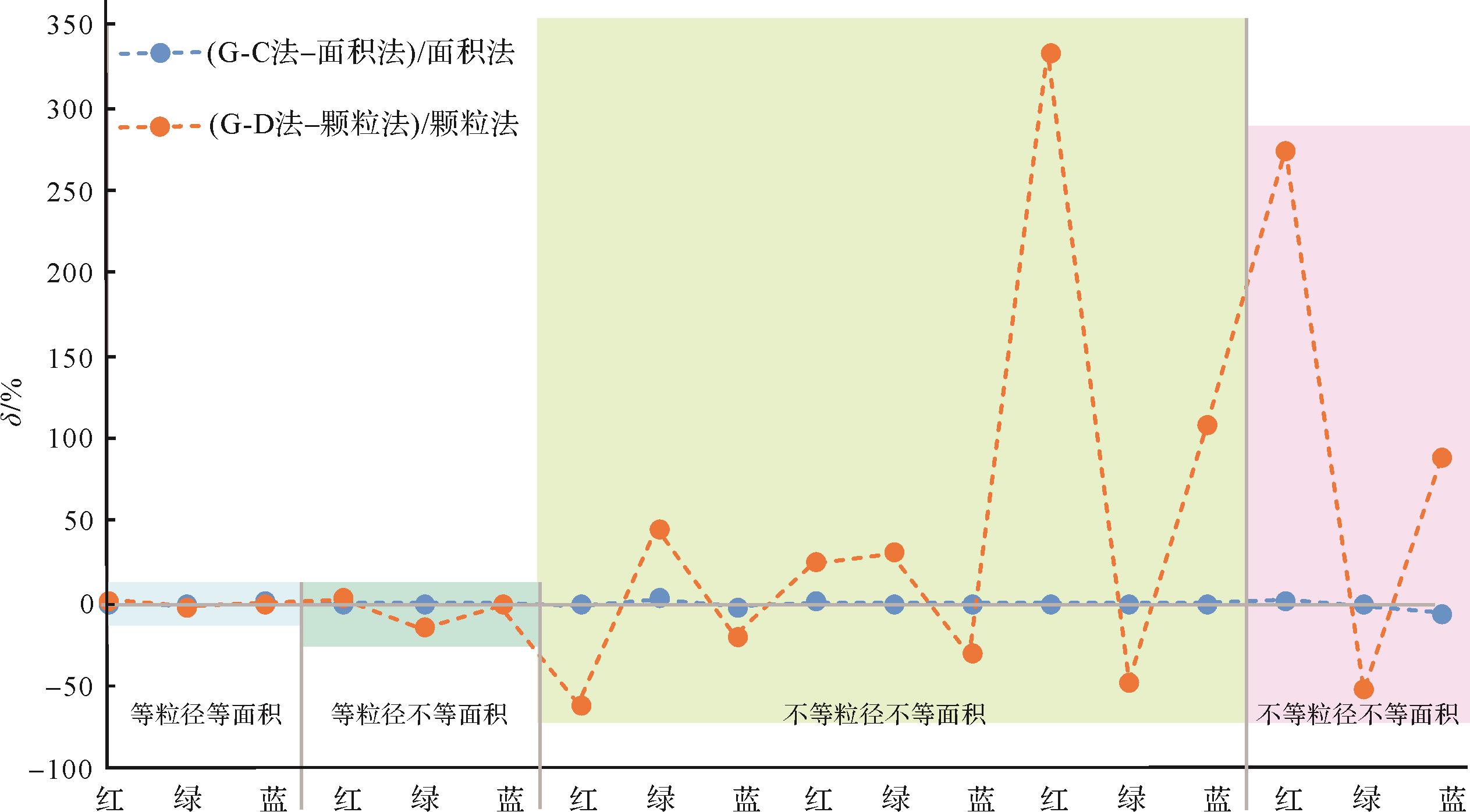
  • 用Matlab模拟采用全颗粒法与Gazzi-Dickinson方法对等粒径等面积、等粒径不等面积、不等粒径等面积和不等粒径不等面积四种情况下的红、绿、蓝三色小球进行统计,在等粒径的条件下两种方法的统计结果相近,偏差最大为15%,其他均小于5%;在不等粒径的条件下两种方法的偏差最大可达333%(图8)。说明在分选较好时,全颗粒法与Gazzi-Dickinson方法统计结果相近,在分选较差时,两种方法的统计结果偏差较大,Gazzi-Dickinson方法统计结果并不能完全代表全颗粒法统计结果。

    Figure 8.  Deviations of the two statistical methods for different scenarios (red, green and blue=three grain types)

    实际统计表明Gazzi-Dickinson法与全颗粒法存在一定的偏差,这种偏差是由于统计方法本身的差异所造成的,而模拟统计均表明在等粒径条件下Gazzi-Dickinson方法与全颗粒法统计结果偏差较小,在不等粒径条件下两种方法的统计结果偏差较大。

  • 两个样品中,全面积法与Glagolev-Chayes方法的统计结果相近,样品16A063的偏差范围为-21%~22%,样品16A064的偏差范围为-14%~5%(图7b1,b2、表2)。两个样品均表明无论是大类还是小类,两种方法的统计结果较为相近。

  • 模拟采用全面积法与Glagolev-Chayes方法统计,无论是等粒径还是不等粒径,两者的统计结果相近,偏差小于2%(图8)。

    实际统计和模拟统计都表明Glagolev-Chayes方法和全面积法的偏差较小,可以认为Glagolev-Chayes方法是全面积法的等效替代。

  • 两个样品均表现出全颗粒法与全面积法的统计结果有较大的差异,样品16A063的偏差范围为-83%~92%,样品16A064的偏差范围为-52%~27%。样品16A063的分选较差,相较而言,样品16A063采用全颗粒法和全面积法统计的偏差更大。说明样品的分选越差,全颗粒统计法和全面积法统计结果的差异性越大(图7c1,c2、表2)。

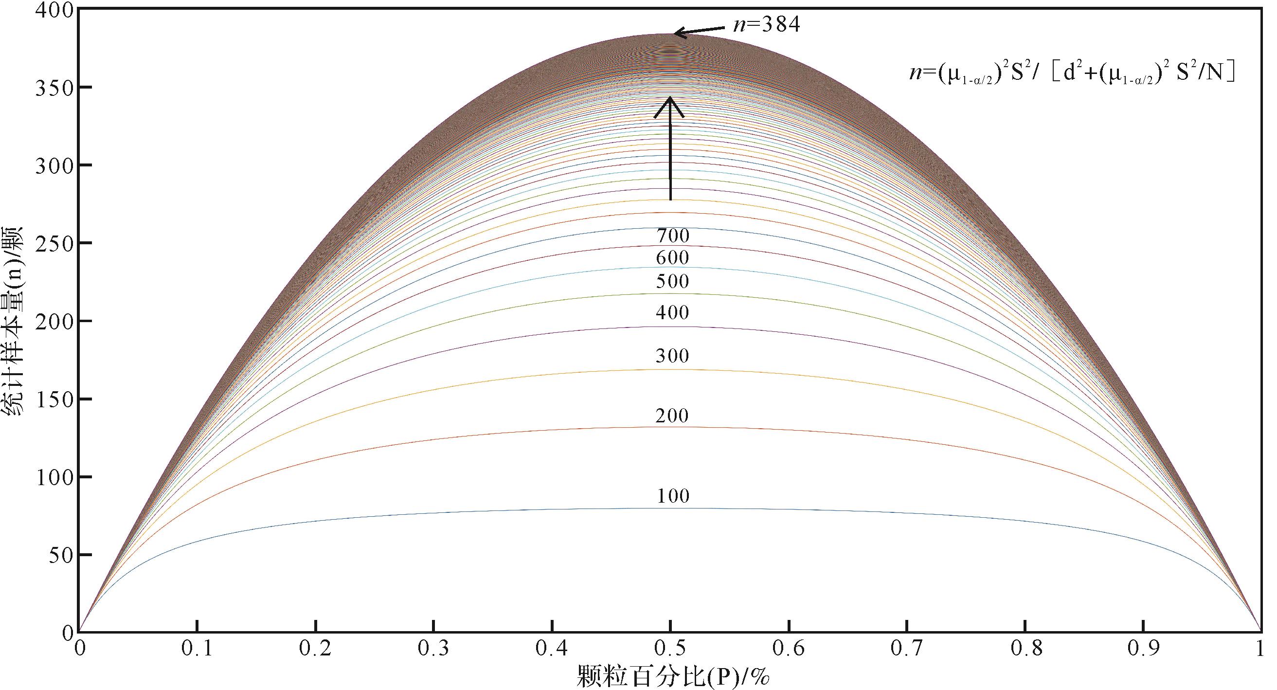
  • 将碎屑统计认为是抽样统计,对于随机分布的总体,按照绝对精度决定样本量n的公式为:

    n=(μ1-α/22S2/[d2+(μ1-α/22S2/N]

    式中α为显著性水平;μ1-α/2是N(0,1)分布的1-α/2分位数;S2为总体方差,S2≈P(1-P);d为绝对精度(绝对误差);N为样品总数,P为颗粒百分比[3132]

    当α取0.05时,达到置信度为1-α=95%,此时μ1-α/2=1.96;当P取0.5时,有最大总体方差0.25,d为绝对精度即绝对误差,一般取5%。可得到随着颗粒百分比的含量的增加,以及总体数量N的增加,所需抽样的样本容量曲线(图9)。

    Figure 9.  A reference chart for the number of detritus statistics

    当样品总数N不断增加时,所需抽取的样本量n也不断增加。当N趋于无穷大时,抽样数n为定值,此时:

    n≈(μ1-α/22S2/d2

    代入上式得:

    n≈(1.96)20.5(1-0.5)/0.052≈384

    所以对任意的样品,抽取的样本量达到384以上时,达到95%的置信度。

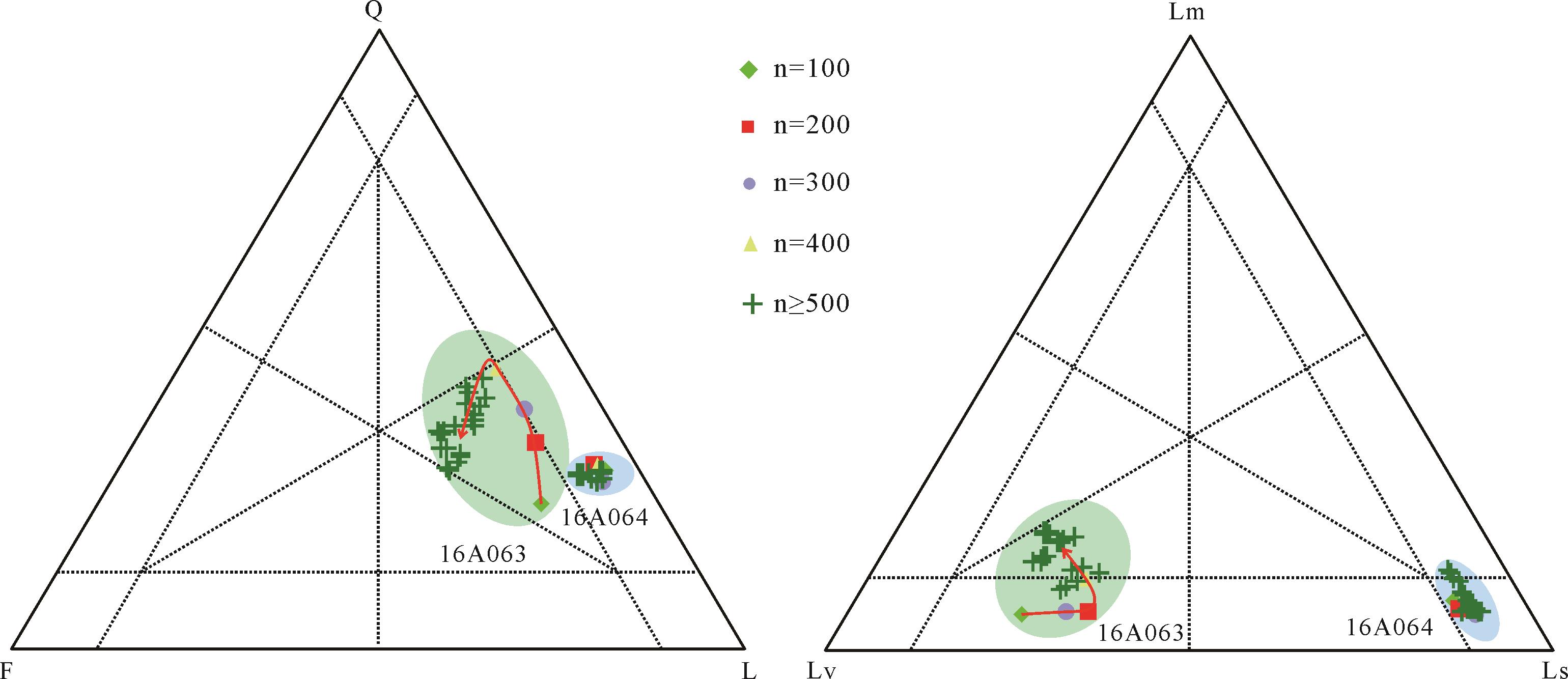
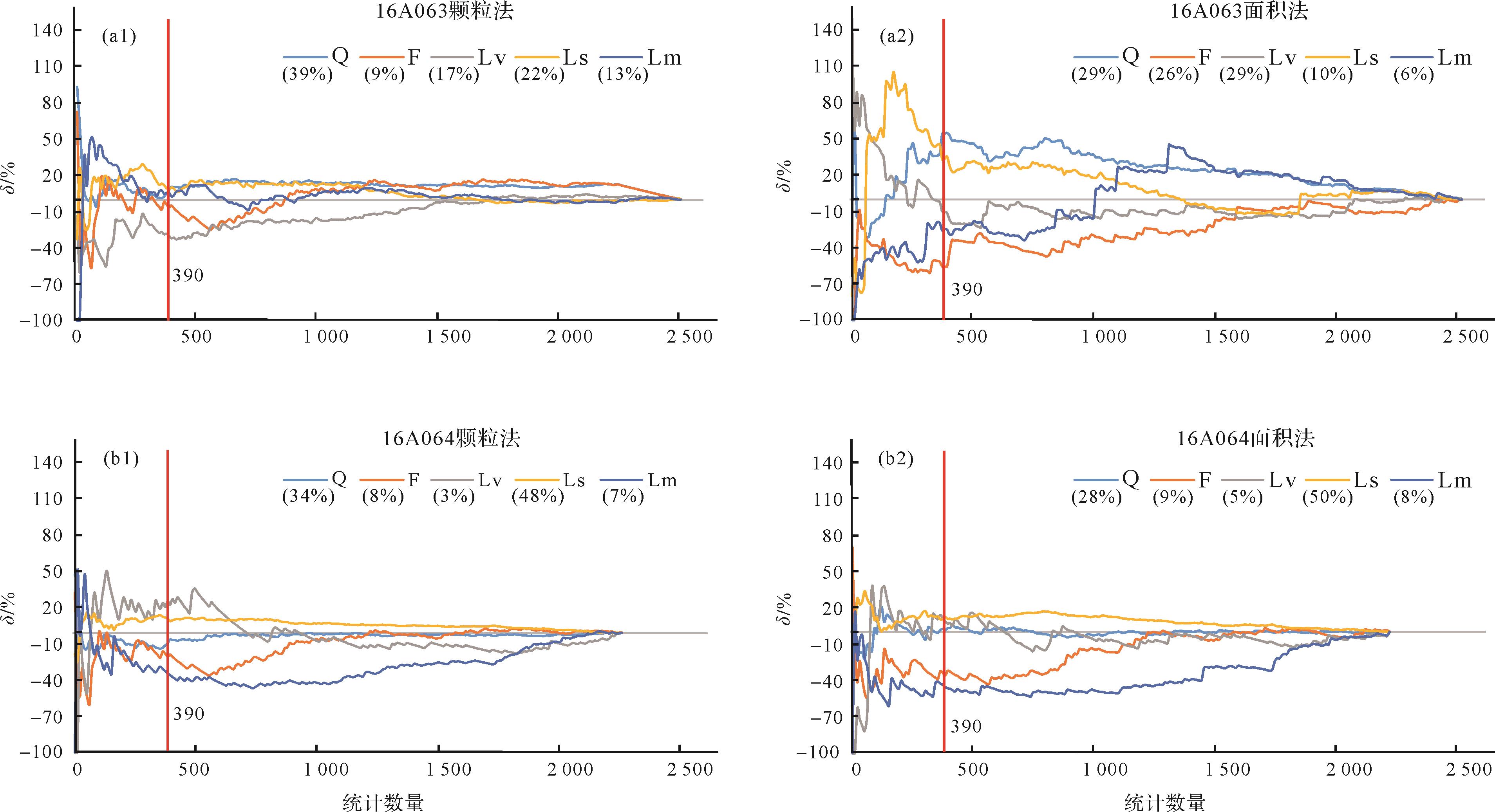
    这个理论计算的数量是否符合实际样品的统计呢?我们将实际统计的两个样品进行验证。将面积法统计结果按照100为公差累积统计,进行三角投图。从图10中可以看出,对于样品16A063来说,前400颗的统计偏差较大,而超过400颗后统计结果偏差相对较小,落点均位于同一岩性内。样品16A064投点均比较集中。

    Figure 10.  Incrementing statistical cast with 100 tolerances

    将样品16A063和16A064采用颗粒法和面积法统计的统计结果以10为公差的累积计算,将含量<5%的颗粒类型与相似参数进行合并,共分为5类。以最终统计的结果作为标准,将其他各数量的统计结果与该标准求偏差。采用颗粒法统计时,样品16A063前200颗的偏差范围最大为-100%~92%,当统计数量达到390颗时,各类型颗粒偏差范围降低至-30%~6%。样品16A064的统计结果与16A063相似,统计390颗以上F/Lm/Lv偏差依然较大,是由于颗粒本身的含量较低导致的(图11a1,a2)。采用面积法统计时,样品16A063总体偏差范围较大为-100%~158%,是由于样品分选较差所造成的。统计390颗以上偏差范围减小至-25%~55%,样品16A064的统计结果与16A063相似(图11b1,b2)。

    Figure 11.  Samples 16A063 and 16A064 using the area method and the point⁃counting method with tolerance of 10 for cumulative statistics

    总体而言两个样品在统计390颗以上时,各类型的统计结果与最终统计结果的偏差较小,且较为恒定,个别偏差依然较大的与颗粒含量较低有关。所以理论计算出的384颗与实际统计结果相一致,且该统计数量不受颗粒分选的影响,是一个可行的统计数量。

  • 两个样品统计结果表明,全颗粒法与全面积法的统计结果有较大的偏差,且样品的分选越差,两种方法统计结果的偏差越大。样品16A063的分选程度差于样品16A064,颗粒法与面积法统计的偏差前者大于后者(图7c1,c2)。

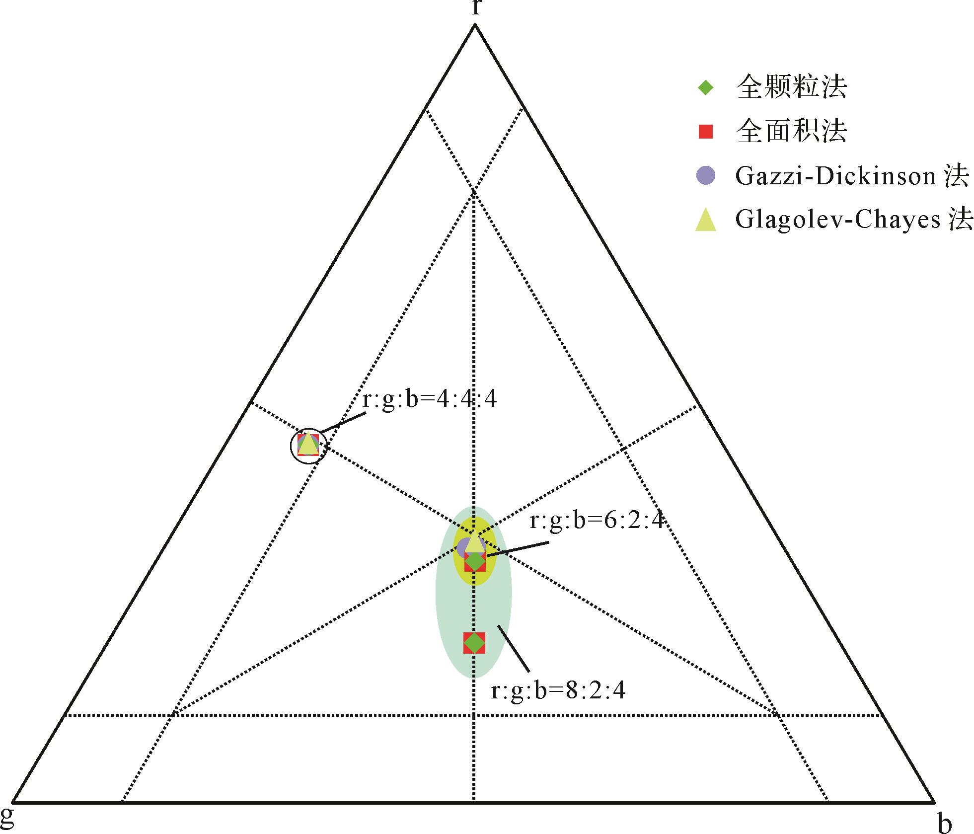
  • 设置红(r)绿(g)蓝(b)三种不同颜色的球,分为三种不同的粒径组合和含量,分别为:1)等粒径不等面积,粒径比r∶g∶b=4∶4∶4;2)等面积不等粒径,粒径比r∶g∶b=6∶2∶4;3)等面积不等粒径,粒径比r∶g∶b=8∶2∶4。三种不同分选的情况分别采用四种不同的统计方法统计1 900颗以上,将统计结果进行三角投图比较。随着颗粒分选由好到差,四种方法的统计结果的投图分散程度变大(图12)。

    Figure 12.  Simulation of the different results affected by grain sorting

    说明利用不同的方法对不同的分选程度的样品进行统计时,碎屑颗粒分选越差,由此造成的面积法和颗粒法统计结果的差异性也会更大,所得到的统计结果差异性越大,投点也更分散。

  • 当某种颗粒类型的面积百分含量或者颗粒百分含量小于样品的10%时,则将该类型颗粒认为是“短板”,既可以是大类,也可以是小类。

    采用颗粒法和面积法两种方法所得的统计结果中,含量小于10%的颗粒类型的统计值偏差波动范围变化大,如采用颗粒法统计时样品16A063中的长石颗粒(F),样品16A064中的F/Lv/Lm(图10a1,a2、表2);采用面积法统计时样品16A063中的Ls/Lm,样品16A064中的F/Lv/Lm(图10b1,b2、表2)。其他类型的颗粒也有较大的偏差,但其波动范围较小。

  • 设置等粒径和不等粒径两种情况,以验证在这两种情况下“短板”现象是否均存在。采用Gazzi-Dickinson法对等粒径颗粒统计,设置绿球的面积百分含量为3%,所得到的统计结果与已知面积求得相对偏差,绿球偏差达10%~20%;对不等粒径统计时,即R(r)∶R(g)∶R(b)=2∶4∶3,颗粒比为n(r)∶n(g)∶n(b)=11∶70∶19,令红球的面积百分含量为10%,含量相对较少的红球和蓝球均有较大的偏差达5%~25%(图13a,b)。

    Figure 13.  Simulation of the “short board” phenomenon for Gazzi⁃Dickinson method and Glagolev⁃Chayes method

    采用Glagolev-Chayes法统计,设置等粒径,令蓝球的面积百分含量为9%,所得到的统计结果与已知面积求得相对偏差,蓝球的统计含量相对偏差为2%~12%。设置不等粒径即R(r)∶R(g)∶R(b)=8∶2∶4,颗粒比为n(r)∶n(g)∶n(b)=10∶160∶1,设置蓝球的面积百分含量为2%,蓝球统计相对偏差为10%~40%(图13c,d)。

    采用Gazzi-Dickinson法和Glagolev-Chayes法统计均存在“短板”现象,且含量越低偏差越大。当统计数量少于500颗时,这种现象更为显著。

    在展示结果时,要把这些“短板”非常明显的颗粒类型进行重点考虑,如果统计的颗粒为384颗时,则不能将这些短板的参数直接使用,例如对于Q/F/L三个参数来说,如果L<10%,则L不宜再细分,不应进行Ls/Lm/Lv分析。可与相类似的参数进行合并,以避免“短板现象”的出现。如果重点关注这种短板类型的颗粒,则需要统计更多的数量才能得到较为准确的比例。

  • (1) 采用颗粒法和面积法对同一样品进行统计时,两种方法的统计结果有较大的偏差,且样品分选程度越差,两种方法的统计结果偏差越大。

    (2) Gazzi-Dickinson法并不能代表真实的面积比,Glagolev-Chayes法是对面积的等效替代。

    (3) 在统计过程中如果某种类型的颗粒含量小于10%,则认为该类型颗粒为“短板”,应该将其与相似的参数合并。如果重点关注该类型,则需要统计更多数量的颗粒。

    (4) Gazzi-Dickinson法适用于物源分析,而进行物质通量计算时,推荐采用Glagolev-Chayes法或面积法进行碎屑统计。统计数量至少达到384颗。

Reference (32)

Catalog

    /

    DownLoad:  Full-Size Img  PowerPoint
    Return
    Return